
By: John Bielinski, Ph.D.
The central purpose of a score on any classroom assessment is to convey information about the performance of the student. Parents, educators and students want to know whether the score represents strong performance or is cause for concern. To valuate a score, we need a frame of reference. For example, it is not enough to say Ian earned a score of 64. We need to know how that score compares to expectations. While there are many ways to define expectations, our instinct is to use what we know about the student’s peer group’s performance. The teacher, who knows the performance of the entire class, might recognize that a score of 64 is above average.
Norms and Percentiles
Whether we realize it or not, our tendency is to characterize all measurable traits normatively. This natural tendency is one of the reasons why normative scores are so useful for describing academic performance. A norm can be thought of as the characterization of the typicality of a measured attribute in a specific group or population.
Here we will limit measured attributes to test scores. The measurement of performance begins as a raw score – such as the total number correct. Then, the score needs to be translated into a scale that indexes what is typical. An especially convenient and readily understood scale is the percentile rank.
A percentile represents the score’s rank as a percentage of the group or population at or below that score. As an example, if a score of 100 is at the 70th national percentile, it means 70% of the national population scored at or below 100. Percentiles generally range from one to 99, with the average or typical performance extending from about the 25th to the 75th percentile. Scores below the 25th are below average and scores above the 75th are above average.
Although percentiles are familiar and are frequently used in educational settings, we rarely consider the development and underlying properties of percentiles. We will briefly examine three aspects of percentiles that contribute to their quality and interpretation, to provide a basis for understanding why national norms in the Formative Assessment System for Teachers (FAST™) were updated and how the update compares to prior norms.
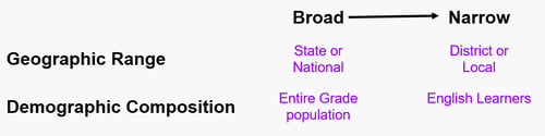
The Reference Group
As stated above, norms are necessarily interpreted in relation to a reference group or population. Yet, we rarely consider the who composition of the reference group beyond general terms such as national or local. But, the composition of the norm group, the demographic characteristics of the group, is essential. The greater the precision with which the group can be defined, the more meaningful the interpretation of the normative scores like percentiles.
The figure below shows examples of reference groups based on geographic range and demographic composition on a continuum from broad to narrow. National norms are typically broad with respect to geographic range and demographic composition. However, there are instances in which local or national norms may be based on a subset of the student populations such as English learners (EL). What is important is that the norm group is well-defined along these dimensions.
The technical documentation for the new FAST national norms provides a detailed description of the demographic composition of the norm groups and how they compare to the entire U.S. school population in each grade. By closely matching the percentages of the U.S. school population by gender, race/ethnicity and socio-economic status (SES) in each grade for each assessment individually, we can accurately generalize performance on FAST assessments relative to the national school population. Another positive consequence of carefully matching demographic percentages is that the norms are stable across grades — they are less prone to possible biasing effects of varying composition, especially relative to SES across grades. The prior FAST national norms also had broad geographic and demographic composition but were not as tightly defined relative to demographic percentages.
The Reference Group
Sample Size and Demographic Matching
Another important characteristic is the size of the norm group. Norms become more stable as sample size increases. What this means is that if we were to compare percentiles derived from many random samples from a population, the score associated with each percentile will vary somewhat across samples. That variability tends to be smaller near the middle of the percentile range (25th – 75th percentile) compared to the tails of the range (1st – 10th and 90th – 99th percentile). This effect can be easily seen through differences in local norms for a given grade across years.
Importantly, sample size does not ensure accuracy. Accuracy refers to how closely the norms match the true population values that would be obtained if they were based on the scores from all U.S. students. To demonstrate the role of demographic match and sample size on accuracy and stability we simulated score distributions that closely match the words per minute (wpm) oral reading rates in Grade 2 on CBMreading for two conditions: sample size (500, 1,000, 2,000, 5,000, 7,000, 10,000) and SES (matched to U.S. and higher than U.S.).
The results are displayed in the figure below. The horizontal lines represent the wpm score associated with the 40th national percentile (some risk cut score). The orange line is the High SES sample and the teal line is the Matched SES sample. Because the teal line is matched to the population, it also represents the true score. For the High SES group, we simulated an effect size bias equivalent to one-tenth of a standard deviation, which is a very small effect. The vertical lines represent the amount of variation in the score associated with the 40th percentile across samples. The longer the vertical line, the more variation and less stability.
Note that the vertical lines are very small with all samples. At 5,000 the instability is equivalent to only one word per minute! This is a negligible effect. Additionally, the worst-case scenario for the Matched SES group, which is the top or bottom of the vertical line at each point, is always better than the best-case scenario in the High SES group.
Two conclusions can be drawn from this simulation. First, a norm sample of 5,000 is sufficient to generate highly stable results. Second, demographic matching can be more important than sample size for samples as small as 500.

Relationship Between Percentiles and Ability
A third property of percentiles that is important to consider when comparing performance across students or comparing the prior FAST norms to the new demographically matched national norms is the nonlinear relationship between percentiles and ability. The blue curve in the figure below shows the relationship between percentiles (vertical axis) and CBMreading wpm scores. The curve is S-shaped and not linear. What this means is that for a given difference in ability (e.g., 10 wpm) the difference in the percentile varies depending on the position in the percentile range.
The dashed lines represent a 10-point difference in wpm. For oral reading rates a 10-point difference is nearly trivial and in fact, it corresponds to the amount of random error present in each student’s score. Thus, a 10-point difference may be no more than random error.
A score of 100 wpm corresponds to the 39th percentile and a score of 110 corresponds to the 49th percentile — a 10 percentile point difference! Whereas the difference between a score of 30 wpm and 40 wpm represent just a two-point percentile difference.
When comparing the new demographically matched FAST norms to the prior national norms, the differences in ability levels for a given percentile are generally small. For CBMreading, Grades 2 – 6, the score differences across the some-risk segment are all less than 10 wpm, while in the high-risk segment the score differences range from seven to 14 wpm. A similar pattern occurs with other FAST assessments. Although these differences are real and will generally result in a smaller percentage of students flagged as at-risk, they should be interpreted in light of the ability difference and not the number of percentile points. As demonstrated here, interpretation of the size of percentile differences depends on the point along the ability continuum the difference occurs.